 Tako Docs
Inspect Cube and Grid Data
On this page
The Cube layer panel renders a scalar field but does not determine its scientific meaning. Before choosing a surface, identify whether the cube stores density, orbital amplitude, spin density, potential, RDG, signed density, a derivative, a reactivity descriptor, or ELF. Field theory and Tako’s fixed generated grid are documented in Density Fields, NCI Analysis, and Volumetric Data.
Open a cube artifact
Open a .cube artifact in Explorer. The viewer parses its title, comment, role metadata, origin, three voxel vectors, shape, atoms, scalar values, minimum, and maximum. Generated Tako comments contain tako_cube_role, which supplies labels such as NCI Signed Density Cube.
The panel initially shows surface controls and grid metadata:
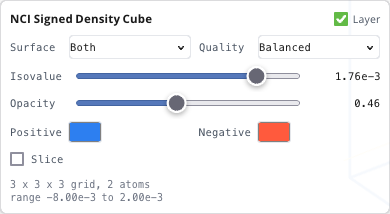
Use the Layer switch to hide or show the active surface without closing the artifact.
Choose surface sign
Tako builds an isosurface with marching cubes, interpolating between voxel samples.
Surface offers Positive, Negative, or Both according to the data range. The same positive magnitude is used for both signs — appropriate for signed orbital amplitude, spin density, potential, charge field, and signed descriptors, while a nonnegative density or RDG normally has only a positive surface.
| Field | Usual surface policy |
|---|---|
| electron density, orbital density, RDG, ELF | Positive |
| molecular-orbital amplitude | Both; colors distinguish phase sign |
| spin density, charge field, potential, Laplacian, dual descriptor | Positive, Negative, or Both according to the question |
| NCI signed density | normally a color field for an RDG surface, not the surface itself |
Opening an artifact automatically chooses Both for signed data, Negative for negative-only data, and Positive otherwise. Other viewer state can persist from a previously opened cube.
Set the isovalue
Isovalue defines the scalar magnitude of the isosurface. The displayed number is authoritative for the view. Signed or high-dynamic-range data use a logarithmic slider spanning four decades below the maximum; other data use a linear slider.
The automatic value is field-agnostic: 22% of maximum absolute value for signed data, or minimum plus 28% of range for unsigned data. It is not a literature threshold. Record the value and test sensitivity.
Do not compare images at “the same slider position.” Compare explicit isovalues in compatible units and model protocols.
Set opacity, colors, and quality
Opacity ranges from 0.05 to 0.95. It changes visibility, not the field. The default is 0.46.
Positive defaults to blue and Negative to orange-red. Color names carry no universal physical meaning; define them in captions. When Map colors is available, select a sibling cube to color the current surface by another scalar field, sampled in world coordinates through a percentile-limited range — approximately the 2nd–98th percentiles for unsigned data and a symmetric ±98th percentile of absolute value for signed data — so each artifact receives a relative color scale, not shared physical units, and the viewer shows no physical color legend. Verify identical origin, axes, and shape first. The viewer does not enforce compatibility and clamps samples outside the companion domain to its boundary.
Quality offers Fast, Balanced, and Fine marching-cubes budgets. It can decimate large imported grids. Tako-generated cubes remain below every budget, so quality does not alter their cell stride or scientific resolution.
Enable a section or clipping plane
Select Slice to expose the plane controls.
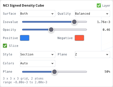
Choose Style:
| Style | Result |
|---|---|
| Section | shows an interpolated scalar plane |
| Clip surface | removes surface geometry on one side of the plane |
| Section + clip | combines the two views |
Axis is Cartesian X, Y, or Z. Plane is a fractional position from 0% to 100% across the grid. With clipping enabled, Keep Below/Above refers to coordinate side, not scalar sign or magnitude.
Colors offers Auto, Viridis, Diverging, and Grayscale. Auto is diverging only when the complete cube range includes both signs. The rendered section is opaque, and its color ranges are percentile-limited and relative to the current cube. The viewer provides no physical legend, so capture range and units separately.
Read dimensions and range
The panel reports Nx x Ny x Nz grid, atom count, and scalar minimum/maximum. It does not display origin, voxel vectors, spacing, geometry units, scalar units, or integration. Use the cube header or tako.cube.parse for those values.
For Tako-generated fields, origin/axes/atom coordinates are stored in bohr and parsed to ångström. Scalar units depend on role and are not converted. Common examples are e bohr for density/signed density, dimensionless for RDG and ELF, and orbital-amplitude units for molecular orbitals.
Pin and compare cube layers
Right-click a cube artifact and choose Pin as layer when several fields must remain available. Keep surfaces sparse enough to remain legible. When mapping one cube onto another, use siblings from the same calculation unless alignment was independently proven.
Viewer controls are global/persisted rather than reset for every artifact. After switching cubes, verify surface sign, isovalue, opacity, colors, map source, slice, and plane. A carried-over setting records nothing about how the current cube was generated.
Build an NCI surface
Requesting NCI cubes from Single Point returns a paired nci_rdg.cube and nci_sign_lambda2_rho.cube. The conventional NCI visualization is one reduced-density-gradient (RDG) isosurface colored by signed density, not two independent surfaces, so build it deliberately rather than opening either cube alone.
Open nci_rdg.cube first. Do not begin with nci_sign_lambda2_rho.cube: opened by itself it produces positive/negative signed-density isosurfaces, a different visualization from the standard RDG-geometry/signed-density-color pairing. Set Surface to Positive, since RDG is nonnegative, and choose an isovalue deliberately — the automatic unsigned default (see Set the isovalue above) is not the method’s summary criterion () and is not a literature-standard NCI choice. Record the value shown beside the slider with every image.
Set Map colors to nci_sign_lambda2_rho.cube. Both NCI fields come from the same runtime grid, so origin, axes, and shape already align; verify this as with any sibling mapping (see Pin and compare cube layers above) rather than assuming it from the filenames alone. Interpret the diverging colors by region:
| Signed-density region | Topological description | What it does not prove |
|---|---|---|
| negative | , attractive-like density concentration | stabilizing energy or bond strength |
| near zero | diffuse/weak density regime | absence or presence of thermodynamic association |
| positive | , repulsive-like density depletion | a force magnitude or steric-energy decomposition |
Move Isovalue through a reasonable range and check whether the contact topology persists: lower values expand diffuse surfaces and are more vulnerable to box/derivative artifacts, higher values contract or remove weak regions. Quality changes rendering cell budgets only; Tako’s generated grid stays below every budget at full stride, so raising quality does not improve NCI numerical resolution. If a surface reaches the outer box, reject that region — the outer voxel shell has derivative terms forced to zero, not real chemistry.
For the RDG/signed-density equations, the fixed grid, and the nci.summary counters in result.json, continue with Density Fields, NCI Analysis, and Volumetric Data.
Import a Gaussian cube
Choose File → Open and select .cube. Tako creates a structure from the atom records, a synthetic completed single-point workspace, and a cube artifact, then opens it.
Import limitations matter:
- Geometry is always interpreted as bohr and converted to ångström. Negative voxel counts that conventionally indicate ångström are accepted by absolute value but still converted, shrinking the geometry.
- Negative atom-count orbital-dataset extensions are not supported.
- Only the first shape-product scalar values are used; extra datasets are ignored.
- The constructed structure cell uses voxel vector times shape rather than shape minus one, so it is one voxel larger than the sampled endpoint extent.
- The stored artifact kind is generic electron density even when title/comment role detection identifies NCI, ESP, or another field.
Verify atom coordinates, origin, axes, dimensions, and role externally before scientific use. An imported .esp filename is not accepted by the current file chooser even though internal role annotation exists.
Export a cube
With a cube artifact active, choose File → Export Cube. This exports the existing cube text; it does not resample the field, bake viewer colors, apply an isovalue, or export a mesh.
Keep result.json, the matching structure, and calculation settings with the file. A standalone cube header lacks enough provenance to reproduce the electronic model or derivative analysis.
Verify alignment and meaning
Before interpreting or mapping any cube:
- Identify the scalar role from calculation contract and header metadata.
- Verify atom count/coordinates against the source structure.
- Record origin, three voxel vectors, shape, and coordinate units.
- Determine scalar units and whether signs represent phase, spin, charge, curvature, potential, or a descriptor.
- Confirm mapped fields share identical grids.
- Check isosurface/section behavior across stated thresholds.
- Inspect boundaries for truncation or derivative artifacts.
- Keep screenshots secondary to the raw cube and provenance.
Diagnose viewer and import problems
| Observation | Check | Response |
|---|---|---|
| Cube does not open | parser requires header, positive effective dimensions, atom lines, and at least shape-product finite values | validate/repair the file externally |
| geometry is too small after import | negative voxel-count Å convention was misread as bohr | convert header coordinates/vectors to bohr or use an external viewer |
| wrong semantic title/artifact kind | role inference and stored artifact kind differ | trust explicit header/provenance, not generic Explorer kind |
| surface vanishes | sign unavailable or isovalue outside useful range | inspect min/max, choose valid polarity, adjust explicit value |
| mapped colors form edge bands | companion grid is misaligned/out of domain | stop mapping and align/resample fields externally |
| Fast/Balanced/Fine look identical | generated grid is below every decimation budget | expected; quality is not grid resolution |
| new cube inherits odd clipping/color | viewer settings persisted | reset every relevant control manually |
| exported file lacks the visible section/colors | Export Cube writes scalar text, not rendered scene | capture figure separately and document rendering settings |
For programmatic parsing, derivatives, integration, histogramming, and writing, use NCI and Volumetric Data with Tako Script.