Run a Single-Point Calculation

Page type: Task guide

On this page

Open Single Point Setup
Select the calculator state
Select Outputs
Start the calculation
Open the result
Request NCI outputs
Conditional states

Use this procedure to evaluate the active structure without changing its atomic positions or cell. The scientific meaning of energies, forces, stress, and electronic outputs is developed in Single-Point Energies and Properties.

Open Single Point Setup

Activate the structure tab to be evaluated. In the top bar, open Calculate and select Single Point. The Single Point Setup dialog opens; its subtitle identifies the active structure.

In the left tool rail, select Calc, then select Single Point. The same Single Point Setup dialog opens. Both entry points act on the active structure tab.

Select the calculator state

In Calculator, select Model. For a GFN2 model, enter Total charge and Unpaired electrons for the intended electronic state. The additional GFN2 controls—SCF energy threshold, SCF density threshold, SCF max cycles, Electronic temp K, Mixer damping, SCF output interval, and Implicit solvation—appear in the same section.

For an MLIP model, charge, spin, and electronic-analysis controls do not give the structure-only model an electronic state. The dialog disables output choices that the selected model cannot provide and displays the reason below the disabled label.

Static asset requirements and current cache status appear below the calculator fields when the selected runtime or model weights require preparation. Actual download preparation begins after Start. A model that is downloaded is available to load; its presence does not establish suitability for the structure.

Select Outputs

In Outputs, select each required property:

Visible label	Result produced when supported
Energy	Total model energy
Forces	Atomic force array
Stress	Cell stress tensor
Charges	Atomic population analysis
DOS	Electronic density-of-states data
PDOS	Projected density-of-states data
Charge density	`charge_density.cube`
NCI cubes	`nci_rdg.cube` and `nci_sign_lambda2_rho.cube`
WFN	`wavefunction.wfn`

Energy and Forces are the basic fixed-geometry channels. Select other outputs only when the calculator and subsequent analysis require them. Cube and wavefunction outputs can be substantially larger than scalar or tabular results.

Start the calculation

Select Start. Tako closes the setup dialog and creates SP-<N>-calc in Explorer before the numerical work finishes. The folder contains the copied input structure and generated run record under input, while calculation progress, asset-download progress, and diagnostic messages appear in the calculation and Console surfaces.

To leave without creating a calculation, select Cancel. The header close button has the accessible name Close setup and performs the same action.

Open the result

When the workspace completes, expand SP-<N>-calc in Explorer. Open output/result.json for the structured result and output/log.txt for the calculation trace. Requested property artifacts appear beside them, for example charges.json, dos.json, pdos.json, the selected cube files, or wavefunction.wfn.

Open DOS/PDOS, charge, and cube artifacts with their corresponding result views. A plot or isosurface is a view of the stored numerical artifact; retain the artifact and its settings when reporting the result.

A completed workspace means that Tako received a structured result. The geometry is not thereby stationary, and energies are comparable only under a consistent calculator and reference. Inspect the force array, the calculator state, and every requested artifact before using the result.

Request NCI outputs

Select NCI cubes in Outputs to request Tako’s non-covalent interaction (NCI) fields alongside the base single-point result. The option requires a GFN2 or GFN2+D4 calculator; an MLIP model exposes no electron density, so the checkbox is disabled and the dialog states the reason.

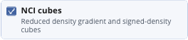
NCI cubes output option showing the exact RDG and signed-density description

Selecting NCI cubes computes the electron density on Tako’s fixed grid and returns two paired cube artifacts:

Artifact	Scalar field	Role
`nci_rdg.cube`	reduced density gradient (RDG), dimensionless	isosurface geometry
`nci_sign_lambda2_rho.cube`	$\operatorname{sign}(\lambda_2)\rho$ , nominal e bohr $^{-3}$	color field for the RDG surface

Both cubes originate from the same runtime grid and are meant to be opened together, not read individually. Because the NCI stage reuses the same GFN2 SCF as Energy and Forces, charge, unpaired electrons, geometry, and implicit solvation all affect the resulting density. There are no visible controls for grid shape, padding, density floor, or isovalue; current values are fixed in the runtime.

Continue with Inspect Cube and Grid Data to pair and render the two cubes, and with Density Fields, NCI Analysis, and Volumetric Data for the RDG/signed-density theory and interpretation limits.

Conditional states

Visible state	Meaning	Action
An output is disabled and explanatory text mentions MLIP	The selected model exposes only structural channels	Select GFN2 when the question requires electronic output, or remove that request
Calculation needs one cell appears	Multiple visible periodic layers have incompatible cells and cannot be submitted as one structure	Compose the visible layers into one consistent cell or hide the layers that do not belong to the calculation
Static model/runtime rows are shown in the dialog	The selected calculator has asset requirements and a current cache state	Review the requirement; after Start, follow actual preparation progress in the calculation/Console UI or use Model Manager beforehand
`SP-<N>-calc` remains failed	Validation, asset preparation, SCF, engine execution, or result publication failed	Open `output/log.txt`; correct the first substantive error before rerunning
Energy is finite but forces are large	The fixed-geometry evaluation completed away from a stationary point	Preserve the result if that geometry was intentional; otherwise run a separate optimization

Tako Script uses a separate contract. See Single-Point Calculations with Tako Script rather than translating this interface procedure field by field.