Calculate Molecular Vibrations

Page type: Task guide

On this page

Structure state before opening the dialog
Open Vibration Setup
Vibration controls
Spectra controls
Start and follow the calculation
Files and viewers
Accepting or rejecting the result
Failure patterns

The Vibration command evaluates the Cartesian force-constant matrix of a finite structure and writes normal modes, signed frequencies, and zero-point energy. With a GFN2 calculator it can additionally evaluate infrared intensities and Raman activities. This page describes the visible controls and resulting workspace files. The derivation and interpretation of the mass-weighted Hessian are given in Molecular Vibrations and IR/Raman Spectroscopy; the JavaScript contract is separate in Molecular Vibrations with Tako Script.

Use this command on a molecule or non-periodic cluster. A periodic crystal requires Calculate Crystal Phonons, because molecular translation/rotation projection and crystal wave-vector sampling are different problems.

Structure state before opening the dialog

Activate the geometry whose Hessian is required. Normally this is the accepted final frame of a converged optimization performed with the same calculator and electronic state. Check the following before starting:

the structure has no accidental periodic cell or periodic-boundary flag;
charge, number of unpaired electrons, dispersion, solvent, and calculator variant match the preceding optimization;
the optimization residual is small enough for the intended frequency accuracy;
constraints are intentional, because completely fixed atoms are excluded from the active atom set; a partially fixed atom remains active;
the atom count is feasible for repeated force and response calculations in browser memory.

The vibration command does not optimize the structure. An imaginary internal mode may therefore describe a genuine saddle, an unconverged geometry, or a numerically poor Hessian; the command itself does not choose among those interpretations.

Open Vibration Setup

In the left tool rail, choose Calc, then Vibration. Tako opens Vibration Setup for the active structure. The upper calculator region is shared with other calculation dialogs. Select the same Model and GFN2 electronic-state fields used to define the stationary geometry; Choose a Calculator documents those controls once.

For frequencies alone, an MLIP or GFN2 model may be used. IR and Raman response are implemented only by the semi-empirical GFN2 path. The IR and Raman cards remain selectable when an MLIP is chosen, but the worker logs that the response is unavailable and does not return those payloads. If spectra are required, select GFN2-xTB and choose dispersion separately before starting.

Vibration controls

Vibration finite-difference controls showing displacement and stencil size

The Vibration region contains the two numerical controls that define the finite-difference Hessian.

Control	Meaning	Current default	Consequence
Displacement A	Cartesian displacement magnitude $\Delta$ in ångström	`0.01`	Each Cartesian coordinate of every active atom is evaluated at $\pm\Delta$ for a two-point stencil, or at $\pm\Delta$ and $\pm2\Delta$ for a four-point stencil.
Finite diff points	Central finite-difference stencil	`2`	`2` uses two displaced evaluations per active Cartesian coordinate. `4` uses four and reduces leading truncation error, but doubles the displaced calculations.

The dialog accepts a positive displacement and offers only 2 or 4 finite-difference points. 0.01 Å is a starting value, not a universal convergence setting. If quantitative frequencies matter, repeat the calculation at a second sensible displacement and compare the internal modes. A result that changes materially with $\Delta$ is not numerically converged with respect to the finite difference.

For $M$ active atoms, the normal-mode pass evaluates the undisplaced structure plus $6M$ displaced structures with the two-point stencil, or plus $12M$ with the four-point stencil. Completely fixed atoms do not contribute displaced coordinates. A per-axis Cartesian constraint does not remove its atom from this active set; its force components are constraint-adjusted, so document partial constraints especially carefully. Requesting IR and Raman currently launches separate finite-difference response passes, so selecting every spectrum can make a GFN2 calculation substantially more expensive than frequencies alone.

Spectra controls

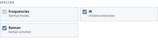
Spectra controls showing mandatory frequencies and optional IR and Raman response

The Spectra region chooses the returned response channels.

Card	Visible state	Returned data
Frequencies — Normal modes	Selected and disabled	Always computes signed frequencies, complex frequency components, vibrational energies, zero-point energy, and mode vectors. It cannot be removed from a vibration calculation.
IR — Infrared intensities	Selected by default; may be cleared	With GFN2, computes dipole derivatives and returns intensities, the static dipole, a response-pass force diagnostic, and its associated modes. With an MLIP, no IR payload is produced.
Raman — Raman activities	Selected by default; may be cleared	With GFN2, computes finite-field polarizability derivatives and returns activities, absolute intensities, and Placzek invariants. With an MLIP, no Raman payload is produced.

Clear IR or Raman when that observable is not part of the analysis. This is a calculation choice, not merely a plot preference: each selected GFN2 response changes the work performed by the backend.

Start and follow the calculation

Press Start after reading the selected model, displacement, stencil, and spectra once more. The setup dialog closes and the calculation console reports distinct stages: vibrational modes, optional infrared intensities, optional Raman activities, and completion. The Explorer calculation folder is created before the worker finishes, so pending files can appear before their payloads are available.

A completed progress message does not confirm that the payloads were produced. Open the calculation record and confirm that the requested result payloads exist. If an MLIP was used with IR or Raman selected, the missing spectrum is an expected capability boundary only when the log explicitly reports that semi-empirical response is required.

Files and viewers

Every successful vibration calculation makes vibrations.json and vibrations.traj available. Additional files depend on requested and supported response:

Explorer file	When available	Opened representation
`vibrations.json`	Frequencies completed	Signed frequencies in cm⁻¹, complex components, energies, zero-point energy, and Cartesian mode vectors derived from the mass-weighted eigensystem
`vibrations.traj`	Mode vectors could be converted to frames	Sixteen display frames per mode for animation; these are visualization displacements, not a molecular-dynamics trajectory
`ir_spectrum.json`	IR requested and returned by GFN2	Frequencies, ASE-convention intensities in (D/Å)² amu⁻¹ despite the historical `intensities_au` field name, static dipole magnitude, and response diagnostics
`ir_modes.traj`	IR payload contains modes	Animated modes weighted for display by relative IR intensity
`raman_spectrum.json`	Raman requested and returned by GFN2	Raman activities, the current duplicate `absolute_intensities` alias, and raw $\alpha^2$ , $\gamma^2$ , $\delta^2$ derivative invariants
`raman_modes.traj`	Raman payload contains modes	Animated modes weighted for display by relative Raman activity

Open a spectrum JSON file to use the spectrum viewer. Open a trajectory and select a mode to inspect the atomic displacement. Tako scales mode vectors to a visible amplitude and assigns a playback interval from the absolute frequency; neither display scaling nor animation speed is part of the computed eigenvector normalization.

Accepting or rejecting the result

For an intended minimum, inspect every materially imaginary internal mode. Very small signed-negative values can result from incomplete removal of translations and rotations, finite SCF noise, or an imperfect stationary geometry; a chemically directed displacement with appreciable magnitude is evidence against a minimum. For a transition-state candidate, require one meaningful imaginary internal mode and verify that its animated displacement follows the expected reaction coordinate.

Check more than the sign count:

Compare the calculator and electronic state with the preceding optimization.
Inspect the residual-force evidence from that optimization.
Animate suspicious modes and distinguish internal motion from collective translation or rotation.
Repeat the Hessian with a second displacement or the four-point stencil when numerical sensitivity could change the conclusion.
Compare spectra only after defining the same geometry, model, charge/spin state, broadening convention, and intensity normalization.

The harmonic output contains no temperature-dependent free energy and no anharmonic correction. The zero-point energy is the backend’s harmonic sum over positive modes, not a complete thermochemical correction.

Failure patterns

Observation	Inspect	Corrective action
Several large imaginary internal modes	Starting geometry and optimization residual	Return to optimization.
Only low-frequency collective negative modes	Mode animation, molecular isolation, displacement sensitivity	Tighten the stationary geometry and compare a second displacement before classifying them.
Frequencies change strongly between `0.01` and another displacement	SCF/force noise or anharmonic sampling	Tighten electronic convergence where available; compare two- and four-point stencils.
IR or Raman files remain unavailable	Selected calculator and console capability message	Use GFN2 for response properties, or report frequencies only.
Calculation cost is unexpectedly high	Active atom count, stencil, selected spectra	Clear unused response cards, use the two-point stencil for reconnaissance, or reduce the active atoms only with scientifically justified complete-atom constraints.
Animated mode looks exaggerated	Viewer scaling rather than Hessian data	Read numerical vectors in `vibrations.json`; animation amplitude is deliberately rescaled.

For interpretation of signed frequencies, mode normalization, IR intensity, Raman invariants, isotope effects, and the harmonic approximation, continue with Molecular Vibrations and IR/Raman Spectroscopy.