 Tako Docs
Choose a Calculator
On this page
Every calculation setup except XRD contains a Calculator section. Select the calculator there before editing operation-specific controls. The selection determines which properties are available, which assets must be present, and whether charge, spin, SCF, and solvation settings affect the run.
Physical approximations and validation limits: Choosing a Method. This page follows the visible interface.
Open a calculation setup
Display the structure to be calculated. Press Calc in the left rail and then press the required operation, such as Single Point or Optimization. The same operations are available under the top Calculate menu.
The setup dialog opens with Calculator above the operation-specific sections. Its subtitle identifies the active structure. If the dialog displays Calculation needs one cell, more than one incompatible visible periodic layer is contributing a cell; hide the unrelated layer or select the intended structure before continuing.
The current new-dialog default is g-xTB with its native DFT-revD4 dispersion. It is a balanced starting point, not a recommendation for every calculation. Select and record the method required by the chemistry and observable.
Select Model
Choose MLIP, DFT, or Tight binding in Theory family, then select the method in Model / level. This two-step control keeps the initial choice short without hiding any registered level.
| Visible entry | Runtime/model role |
|---|---|
| nequix | General Nequix MLIP using nequix-mp-1 weights |
| nequix PFT | Phonon-fine-tuned Nequix option using nequix-mp-1-pft weights |
| NequIP-S | Smaller NequIP OAM model |
| NequIP-L | Larger NequIP OAM model |
| Equiformer direct | Direct-force Equiformer model |
| Equiformer gradient | Energy-gradient Equiformer model |
| g-xTB | General tight-binding method; dispersion selected separately |
| GFN2-xTB | GFN2 electronic method; choose dispersion separately |
| PBE | DFT with geometry-aware molecular or periodic basis selection |
| r2SCAN | DFT with geometry-aware molecular or periodic basis selection |
| SKALA 1.1 | Molecular DFT using the pinned SKALA checkpoint |
Selection does not assert that a model is accurate for the displayed chemistry.
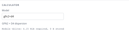
The lines beneath Model are a static readiness summary of the required module and weight asset — not calculation progress, and not a scientific setting.
Read unavailable property states
Property controls respond immediately to Model. In Single Point Setup, an MLIP leaves Energy, Forces, and periodic Stress available; Charges, DOS, PDOS, Charge density, NCI cubes, and WFN are disabled with a reason such as “MLIP only returns energy, forces, and stress.” Select GFN2 when those electronic outputs are required.
A disabled property is a calculator capability boundary, not an unchecked request that can be restored later. Changing the model may also normalize the requested property set, so re-read the output controls after every model change.
Set charge and unpaired electrons
Total charge and Unpaired electrons remain visible in the calculator section. They are operative electronic-state inputs for GFN2. Enter the signed total charge of the complete calculation structure and the intended number of unpaired electrons before pressing Start.
The same fields are visible with an MLIP selected, but the current MLIP inputs are structure-only and do not consume a molecular charge or spin channel. Their presence in the shared form does not indicate MLIP support for redox or spin-state changes. If the scientific comparison changes charge or spin, use an electronic-structure method that represents the required state.
Configure tight-binding dispersion and SCF
Selecting g-xTB displays None, DFT-D3, and DFT-revD4 in the separate Dispersion selector. DFT-revD4 is the native model and default. The DFT-D3 alternative uses published ωB97M D3(BJ) parameters and records that provenance because no separate g-xTB-specific D3 fit is published. Selecting GFN2-xTB instead offers None and its native D4 model.
| Control | Visible purpose |
|---|---|
| SCF energy threshold | Energy-change convergence threshold |
| SCF density threshold | Density-change convergence threshold |
| SCF max cycles | Maximum electronic iterations |
| Electronic temp K | Electronic smearing temperature |
| Mixer damping | Charge/density mixing damping |
| SCF output interval | Interval between SCF log reports |
For an initial calculation we recommend keeping the defaults unless the system or protocol supplies a reason to change them. Increasing SCF max cycles does not repair an incorrect charge, spin state, or geometry. If SCF fails, inspect those physical inputs before weakening convergence.
Expand Temperature annealing to edit Temperature schedule K, Policy, Start temperature K, Stages, and Stage cycles. Expand Advanced SCF to select Initial guess and SCF mixer. Allow unconverged SCF requests a best-effort electronic result; enable it only for explicitly labelled diagnostic work. An unconverged state is not interchangeable with a converged energy in a comparison.
Configure implicit solvation
With GFN2 selected, check Implicit solvation to display Solvation model, Solvent, Electrostatic model, Born kernel, and the available CDS correction, CM5 correction, and Shift correction controls. When Shift correction is checked, Shift state appears.
Solvation changes the energy model and its reference convention; keep it fixed across every term in one comparison (see Preserve comparability below).
Inspect and prepare assets
Open File → Model Manager when the required module or weight is not stored. Press Download for an absent asset; a partial download exposes a resume action, and a cached asset exposes its management action. Closing Model Manager does not select the model — return to the setup dialog and confirm Model again.
Exact identifiers, capabilities, and assets: Calculator Reference.
After Start is pressed, actual asset-transfer and calculation progress appear in the calculation workspace and Console, not the pre-run byte summary under Model.
Preserve comparability
Before starting a series, keep the following fixed unless the change is the subject of the experiment — same calculator, same settings, same charge/spin state:
- the exact Model entry and model asset version;
- Total charge, Unpaired electrons, and dispersion choice for GFN2;
- SCF, solvation, and temperature/annealing settings;
- the requested property set and the operation’s geometry/cell policy.
Full treatment, including why GFN2 and MLIP energies cannot be subtracted from each other: Comparable Energies and Thermodynamic Cycles.
Confirm the selection
Before pressing Start, re-check the model description, required-asset lines, charge/spin fields, enabled output properties, and operation-specific controls. After completion, open result.json and confirm the recorded level of theory, model/runtime, convergence state, and requested outputs. Cache availability means the files can run; target-domain accuracy still requires a matched validation calculation.
Irregular states
| Visible state | Meaning | Action |
|---|---|---|
| Not downloaded in Model Manager | Required asset is absent | Press Download or choose a calculator whose required assets are available |
| Partial asset with resume action | Transfer stopped before completion | Resume the transfer; do not repeatedly restart from a different browser profile |
| Electronic property disabled under MLIP | Selected calculator cannot produce the property | Select GFN2 or change the scientific question |
| GFN2 SCF failure in the calculation log | Electronic state did not meet the SCF contract | Check geometry, charge, unpaired electrons, and physical model before changing numerical controls |
| Plausible but inconsistent energy ordering | Model, state, reference, or geometry policy differs across terms | Rebuild the comparison with one recorded convention |
| MLIP produces an unphysical geometry without an engine error | Structure may be outside the model’s training domain | Reject the result and validate representative configurations against an appropriate reference method |