Agent Demo: Water Stretch–Bend Surface

The question

A water molecule vibrates constantly, but it has a preferred shape: an equilibrium O–H bond length and an equilibrium H–O–H angle. Push in on the bonds or force the angle open and the energy rises. This study maps that rise — not the single number for the resting geometry, but the neighborhood around it: how the energy changes as both O–H bonds stretch together and as the H–O–H angle opens or closes.

The instruction to the agent, in plain words: map how water’s energy changes as its two O–H bonds stretch and its bond angle opens and closes, and show me where the energy is lowest.

Two coordinates, then: a symmetric O–H stretch we’ll call $r$, and the H–O–H bend we’ll call $\theta$. Everything else about the molecule (the antisymmetric stretch where one bond grows while the other shrinks, any twist out of the plane, and where the molecule sits or points in space) we hold still, so what comes back is a clean two-dimensional slice through water’s full energy landscape rather than the whole thing at once.

The agent proposes a plan before writing anything

Working this way, the agent shows its reasoning before it writes code. It came back with a plan we could sign off on:

• Sample, don’t relax. Lay down a grid of fixed geometries and compute one energy at each — a screening scan. No optimization, so every point is exactly the geometry we asked for.
• A 9×9 grid. Nine O–H distances from 0.80 to 1.20 Å in 0.05 Å steps, crossed with nine H–O–H angles from 80° to 160° in 10° steps. That’s 81 geometries, and the ranges deliberately straddle water’s real geometry (about 0.96 Å and 104.5°) so the minimum should fall inside the grid with room on every side, not pinned to an edge.
• One method, everywhere. A single GFN2-xTB calculator, evaluated once per geometry, so all 81 energies are directly comparable. Water is three atoms, so 81 single points is a minute or two of local computation — cheap enough to just do.
• Read it relative. Report every energy against the lowest point on the grid, in kcal/mol, so the surface is easy to read.

That matched what we were after, so we let it write the script.

Building the geometries

The first thing the agent needs is a way to turn the two knobs — a distance $r$ and an angle $\theta$ — into three actual atoms in space. It wrote a small trigonometric helper that does exactly that: oxygen at the origin, and the two hydrogens placed symmetrically so that each O–H bond is exactly $r$ and the angle between them is exactly $\theta$.

function waterAtGeometry(rAngstrom, thetaDegrees) {
  const halfThetaRad = (thetaDegrees * Math.PI / 180) / 2;
  const hx = rAngstrom * Math.sin(halfThetaRad);
  const hy = rAngstrom * Math.cos(halfThetaRad);
  return tako.structure.Atoms(['O', 'H', 'H'], {
    positions: [[0, 0, 0], [hx, hy, 0], [-hx, hy, 0]],
  });
}

Splitting the angle in half and mirroring the two hydrogens across the $y$-axis is what guarantees a symmetric stretch: both bonds always share the same length $r$, and the bisector always points the same way. This is the geometric definition of the slice we chose — a clean symmetric-stretch/bend cut through the landscape, with the asymmetric motions left out on purpose.

Sweeping the grid

With the builder in hand, the rest is mechanical, and the agent kept it that way. It creates one tako.calculator.gfn2() — neutral, closed-shell water with its default settings — and reuses it for every geometry, so nothing about the method drifts as we move across the grid. Then it walks the 9×9 grid, and at each cell it builds the geometry and asks for a single GFN2 energy:

const structure = waterAtGeometry(bondLengthsAngstrom[col], anglesDegrees[row]);
const result = await tako.singlePoint(structure, singlePointOptions);
rowEnergies.push(tako.analysis.energyEv(result));

Eighty-one geometries in, eighty-one energies out — one energy per fixed geometry, no relaxation, all from the same calculator. The agent stores them as a matrix laid out with angle down the rows and bond length across the columns, ready to hand to the plotters.

From raw energies to a readable surface

Absolute GFN2 energies are large, awkward numbers, and on their own they don’t tell you much. What matters is how much more expensive every geometry is than the cheapest one on the grid. So the agent finds the lowest energy it sampled, subtracts it from every point, and converts to kcal/mol:

const minEnergyEv = Math.min(...flatEv);
const zKcalMol = energiesEv.map((row) => row.map((v) => (v - minEnergyEv) * EV_TO_KCAL_MOL));

Now the surface reads like a topographic map: the deepest point sits at exactly 0 kcal/mol by construction, and every other geometry reports how far uphill it is from there. The agent also records which grid node that low point fell on — the coordinates of water’s minimum, as far as this coarse grid can resolve it.

Reading the surface

The agent renders the same relative-energy matrix three ways, each showing a different aspect: a heatmap for a quick read of hot and cold regions, a static contour map for the shape of the basin, and an interactive Plotly surface we can grab and rotate.

All three views agree. There is a single well — one basin, no ridge, no second minimum, no barrier to climb over. The floor of that well lands on an interior node near water’s real bond length and angle, bracketed on all sides by higher-energy neighbors, exactly as the plan intended. Walk away from it in any direction and the energy rises: gently at first, then steeply as you crush the bonds toward 0.80 Å or wrench the angle out toward its 80° and 160° extremes. The highest ground is in the corners, where a short bond and a distorted angle pile on top of each other.

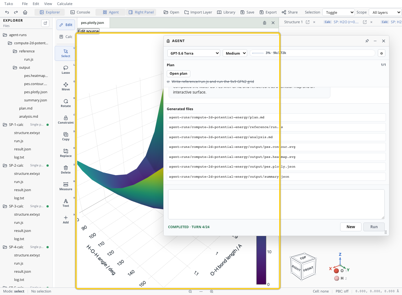
Rotate the surface and the physics is plain: a single potential well with one minimum. That is the shape of a stable molecule — displaced along either coordinate, the energy drives it back.

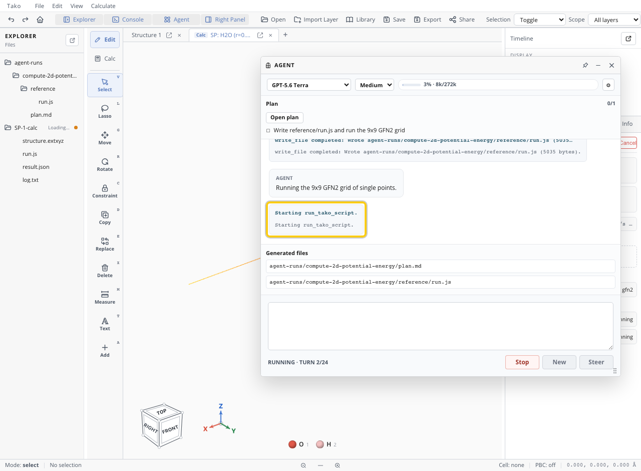
These two screenshots come from Tako’s automated agent-path test, which drives a scripted agent so the run is reproducible in CI; a live agent produces the same script and the same surface — the 81 GFN2 calculations and the plots run for real either way.

What this tells us, and what it doesn’t

The run produced what it set out to find: a picture of water’s energy landscape, confirmation that it’s a single clean well with no hidden barrier, and a good estimate of where the bottom sits — an interior node close to real water’s ~0.96 Å bond length and ~104.5° angle.

One honest caveat, and only one: this is a coarse, unrelaxed screening slice. The grid steps are 0.05 Å and 10°, nothing was optimized, and only the symmetric stretch and bend were allowed to move. So the low point is a well-placed seed, not a converged geometry, and the curvature of this slice is not the molecular Hessian — you can’t read vibrational frequencies off it.

The natural next steps, each handed back to the agent:

• Refine the grid around the basin with finer steps, keeping the coarse scan as context.
• Optimize from the seed — run a same-method geometry optimization starting at the sampled minimum to get a properly converged bond length and angle.
• Confirm with a vibration calculation at that optimized geometry, which turns the well from a picture into real frequencies and verifies it’s a true minimum.

The scan locates the basin; a refinement step pins the exact geometry.

Sources

The automated agent-path test is the source of record for this example. It produces the complete Tako Script and runs the 81 calculations against the real calculation backend. No external experimental geometry or spectroscopic reference is bundled; the numbers come from that run.

For the ideas this scan sits within, see Potential Energy Surfaces for what an energy landscape is, Single-Point Calculations for the per-geometry protocol, Geometry Optimization for turning the sampled minimum into a converged one, and Molecular Vibrations for confirming it with frequencies.