 Tako Docs
Simulate a UV–Visible Spectrum
On this page
The sTDA operation calculates approximate vertical electronic excitations and then samples a Gaussian-folded curve. The controls govern two separate layers: States changes the electronic response solve; E min, E max, Spacing, and Sigma change only the sampled curve. This page describes the interface. The response equations and interpretation limits are developed in Electronic Excitations and UV–Visible Spectra; JavaScript belongs in UV–Visible Spectra with Tako Script.
Prepare the structure
Use the exact geometry, total charge, and unpaired-electron count intended for the vertical excitation. An optimized geometry is often appropriate, but it represents one conformer and one nuclear arrangement. Tako does not optimize an excited state or average a thermal ensemble during this operation.
The backend requires an integral charge and a consistent electron occupation. Charged and open-shell calculations are accepted, but the viewer’s current HOMO/LUMO and S1, S2, … labels are display heuristics rather than validated multiplicity or frontier-orbital assignments.
GFN2-xTB and g-xTB are available. GFN2 is the accuracy-first default for absorption-band positions and uses a dedicated xtb4stda ground-state/response backend. Selecting GFN2+D4 does not add dispersion to a fixed-geometry electronic excitation; calculator solvent, SCF, and mixer settings do not enter that standalone solve. g-xTB is the faster alternative: it runs its normal SCF and passes the accepted orbitals, energies, and occupations directly into the same simplified response kernel. The cached density remains unchanged, and response dipole integrals are evaluated in the calculator-owned q-vSZP basis. g-xTB SCF settings therefore affect the accepted state, while implicit solvation remains unavailable.
Open sTDA Setup
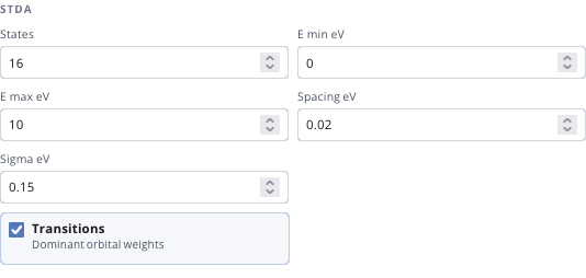
Select the structure, choose Calc, and then choose sTDA. The dialog title is sTDA Setup. The model row starts on GFN2 and also offers g-xTB; the focused sTDA region contains every operation-specific control.
Select response roots
States requests the lowest positive sTDA roots. The default is 16 and the accepted range is 1–256. It does not mean “all states between E min and E max.” The response solver produces exactly the requested root count; the energy window is applied later when the curve is sampled.
Increase States when the highest returned root lies inside or near the spectral region of interest. Continue until peak positions and oscillator-strength distribution in that region stop changing materially. If the selected transition space cannot provide the requested number of positive roots, the calculation fails instead of returning a shorter list silently.
More roots can increase transition-space construction, memory use, and eigensolver cost substantially. Request enough roots to cover the scientific interval.
Set the energy interval
E min eV and E max eV define the energy-domain curve. Defaults are 0 and 10 eV. The minimum is clamped to zero. If the effective maximum is not greater than the minimum, normalization repairs the interval, normally by adding 1 eV.
The interval does not filter states. A state centre outside it remains in the excitation artifact and its Gaussian tail can enter the curve. Conversely, widening E max cannot create omitted high-energy states when too few roots were requested.
Set grid spacing
Spacing eV determines sampling density. The default is 0.02 eV. The interface minimum is 0.001 eV; the lower runtime floors raw requests at 0.0001 eV.
The point count is
There is no point-count cap. An unnecessarily wide interval combined with a fine spacing can allocate a large result array and strain the worker or browser. The final point equals E max only when the interval is exactly divisible by the effective spacing. Reducing spacing samples the same model more densely; it does not improve excitation energies.
Set Gaussian width
Sigma eV is the standard deviation of every normalized Gaussian. The default is 0.15 eV. It is not the full width at half maximum:
The default therefore gives an FWHM near 0.353 eV. Increasing Sigma merges neighbouring sticks and lowers their peaks; decreasing it resolves them and requires sufficiently fine spacing. Sigma is phenomenological broadening. It does not calculate vibronic structure, solvent dynamics, excited-state lifetime, conformer disorder, or instrument resolution.
Keep Sigma fixed when comparing molecules unless changing broadening is itself the analysis. Sigma is a broadening parameter, not a fit parameter for matching experimental envelopes.
Retain transition coefficients
Leave Transitions — Dominant orbital weights selected when state character matters. It retains the four eigenvector components with greatest absolute amplitude for each state. Clearing the switch reduces result detail but does not change energies, transition dipoles, oscillator strengths, or the curve.
Despite the interface wording, returned weight values are signed response-vector coefficients, not normalized percentages. The current compact viewer multiplies them by 100 and sorts by signed value. Read the raw dominant_transitions array for serious analysis; the displayed percentages are not configuration populations.
Start and monitor
Choose Start. The Console reports two coarse stages: solving excited states and building the UV–visible spectrum. The operation does not stream individual states or grid segments. Cancellation terminates the worker and writes no transition-space, eigenvector, or folding checkpoint; a later calculation starts again.
A completed algebraic solve carries no accuracy estimate, so scientific validation remains necessary.
Open the artifacts
The output folder contains result.json, excitations.json, uv_vis.json, and log.txt.
| Artifact | Contents | Use |
|---|---|---|
result.json | full result, duplicated state arrays, curve, effective settings and method labels | provenance and programmatic reuse |
excitations.json | method plus discrete state array | energies, oscillator strengths, transition dipoles and optional coefficients |
uv_vis.json | energy grid, folded intensities and Sigma | curve plotting and downstream processing |
log.txt | progress text | execution record, not scientific state data |
Open uv_vis.json to launch the UV/Vis spectrum viewer. It draws the folded line and sticks, then derives a peak table and state table. The title bar reports point and state counts; the footer reports energy range and Sigma.
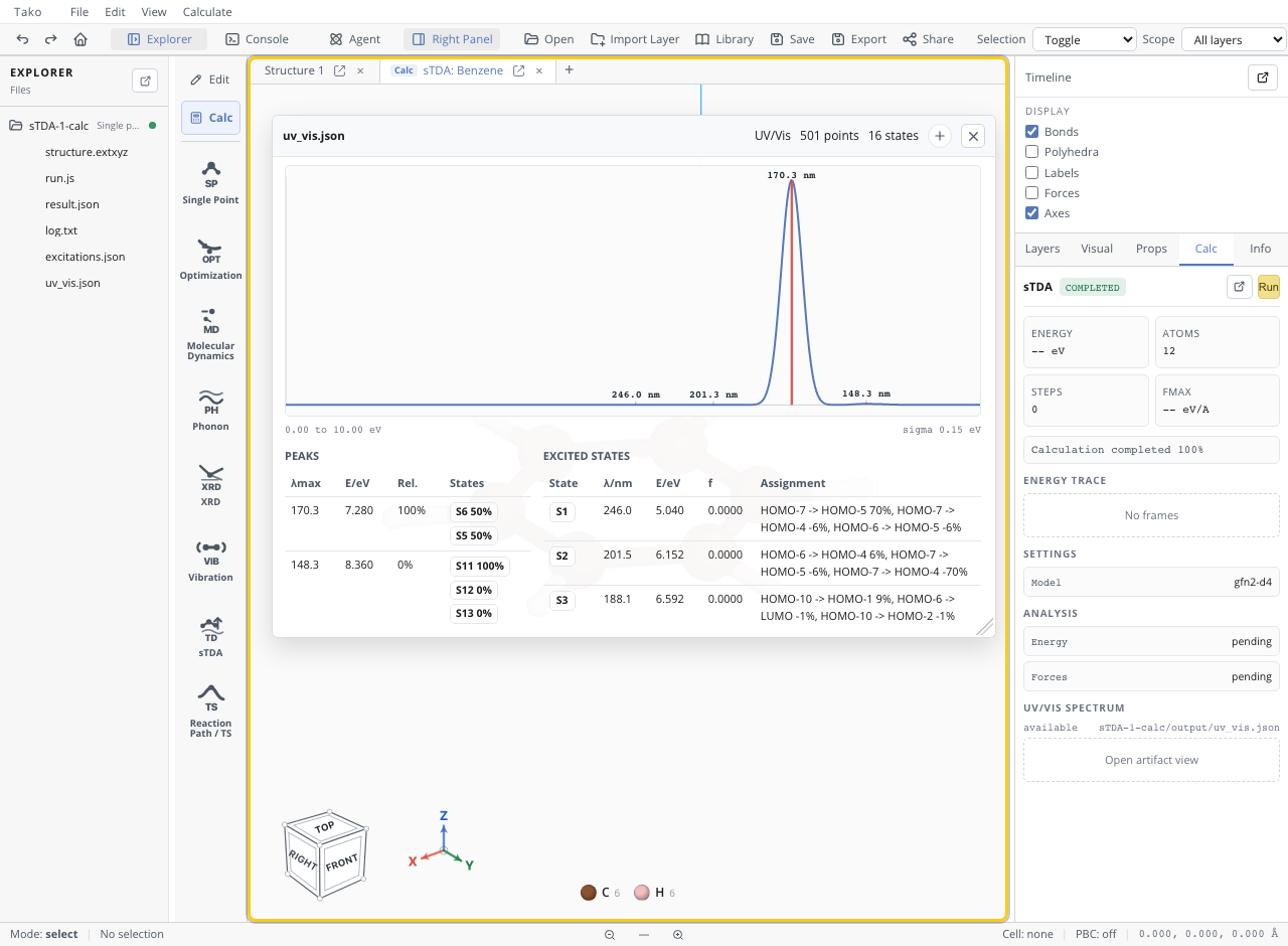
Reading the peak table, the state table, percentage labels, and frontier-orbital heuristics is viewer semantics, not artifact production; see UV–Vis viewer semantics.
Validate the result
- Verify geometry, charge, unpaired electrons, the actual
method("stdaXtb"or"stdaGxtb"), and effective settings inresult.json. - Confirm that the highest root extends beyond the scientific interval; increase States if it does not.
- Inspect discrete energies and oscillator strengths before the broadened envelope.
- Repeat with finer spacing until sampled maxima are stable at the precision reported.
- Keep Sigma and interval fixed for comparative work.
- Test relevant geometries or conformers rather than treating one structure as an ensemble.
- Benchmark representative state types against experiment or a suitable higher-level calculation.
- Record environment differences explicitly; the public operation does not apply selected calculator solvent settings.
The intensity array does not represent molar absorptivity, absorbance, lifetime, fluorescence, excited-state relaxation, or a measured band shape. It is the Gaussian sum of dimensionless oscillator strengths per eV over a finite window.
Diagnose failures and misleading displays
| Observation | Interpretation | Response |
|---|---|---|
| sTDA unavailable | an MLIP or DFT calculator was selected | use GFN2-xTB or g-xTB; document actual method and level_of_theory |
| failure after requesting many roots | too few candidate/positive roots, eigensolver failure, or memory pressure | reduce roots, inspect charge/spin and method domain, then expand cautiously |
| high-energy curve stays empty after increasing E max | too few response roots | increase States, not only the interval |
| peak moves when spacing changes | maximum is selected from sampled grid points | refine spacing and report suitable precision |
| spectrum broadens after increasing Sigma | post-processing changed, not electronic states | compare excitations.json; keep broadening policy fixed |
| transition percentages are negative or omit a major term | signed coefficients are formatted/sorted as percentages | use raw coefficients and rank by absolute magnitude |
| HOMO/LUMO label is implausible | viewer inference ignored charge/spin/model basis | use raw indices and independent orbital analysis |
open-shell states are labeled S1, S2 | viewer uses generic sequential labels | do not infer multiplicity from the label |
| experiment differs systematically | geometry, method, environment, vibronic/ensemble or instrument effects are missing | benchmark the full protocol; avoid an unexplained universal shift |
The exhaustive signature, accepted values, result fields, and normalization behavior are generated in tako.stda Settings.