 Tako Docs
Inspect Spectra and Plots
On this page
Read a plotted artifact as a view of underlying data, with correct axes, units, calculation source, and scientific limitations.
Procedure
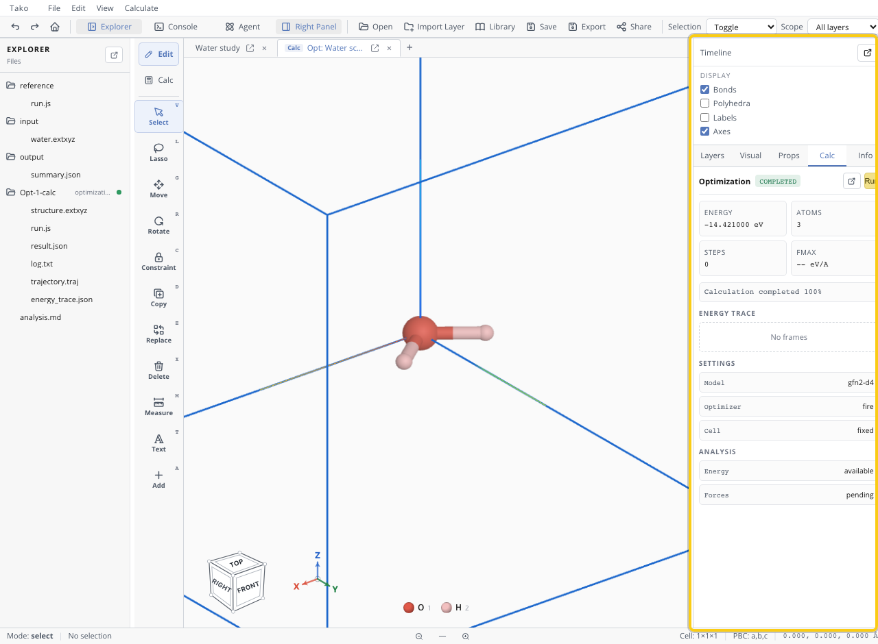
- Open the artifact from its calculation or
output/folder. - Read title, axis labels, units, legend, reference level, and broadening/scaling.
- Locate the raw JSON/CSV that produced the view.
- Use interactive controls only for exploration; preserve the underlying values.
- Compare plots only after aligning method and plotting conventions.
Common plot families
| Artifact | Primary axes/check |
|---|---|
| IR/Raman | Frequency in cm⁻¹; mode/intensity convention |
| Phonon band/DOS | Path/q-point and frequency; imaginary sign convention |
| Electronic DOS/PDOS | Energy relative to Fermi/reference; projection channels |
| XRD | Two-theta and intensity; radiation/wavelength |
| UV-Vis | Energy or wavelength; oscillator strength/broadening |
| Reaction profile | Path/image coordinate and relative energy |
| SVG/Plotly reports | Script-defined units, categories, and source table |
Verify the plot
Confirm raw artifact exists, labels/units match it, reference zero is defined, colors/legends are unambiguous, and no crop hides a load-bearing axis or result. Curve smoothness is set by the broadening, not by numerical convergence.
Troubleshooting
| Symptom | Cause | Fix |
|---|---|---|
| Peak positions differ | Units/reference/model/geometry differ | Normalize conventions before comparison |
| Interactive plot is empty | Invalid/incomplete Plotly JSON | Inspect source file and script log |
| Spectrum is overly smooth | Broadening too large | Inspect sticks/raw states and reduce sigma |
| Axis is cropped | Viewer/window capture issue | Resize/export a complete figure |
| Color implies unsupported ranking | Palette used without uncertainty/evidence | Add values, error/spread, and explicit interpretation |
UV–Vis viewer semantics
Opening uv_vis.json launches the UV/Vis spectrum viewer (see Simulate a UV–Visible Spectrum to produce it). It draws the folded curve and sticks, then derives a peak table and a state table from the raw arrays; the sTDA response theory and folding equations are developed in Electronic Excitations and UV–Visible Spectra. The title bar reports point and state counts; the footer reports energy range and Sigma. The curve, sticks, and any imported reference spectrum are each normalized to their own maximum, so heights compare shape, not a shared absolute intensity scale.
Peak table and “Peaks” chips
The viewer finds sampled local maxima on the folded curve, sorts by height, and keeps at most eight. A boundary grid point can count as a maximum, and peak energy is a grid coordinate — there is no sub-grid fit. Wavelength is calculated as .
The States chips attached to each peak are heuristic: states are selected by proximity within a width derived from Sigma and grid spacing, then their oscillator strengths are normalized into displayed contribution percentages. These “Peaks” and percentages are viewer-derived aids — they are not fields produced by the sTDA eigensolver and not a decomposition of experimental absorbance. For quantitative attribution, calculate contributions from the raw states and the Gaussian folding equation directly.
State table, signed coefficients, and frontier labels
The state table reports a sequential S label, wavelength, energy, oscillator strength , and a compact transition string. The backend does not return excited-state multiplicity or symmetry, so S1 is a row label, not proof that an open-shell state is a singlet. The state detail shows the transition dipole in atomic units — a transition dipole, not the permanent molecular dipole.
Retained transition coefficients (the JSON weight field) are signed response-eigenvector components, not populations. The viewer sorts them by signed value and formats coefficient times 100 as a percentage; a large negative component can therefore be demoted, and labels such as “78%” are not quantitative configuration populations. Use the signed JSON coefficients and rank by absolute magnitude for serious analysis.
Frontier labels (HOMO, LUMO) shown by the viewer are inferred from a HOMO index when one is available. The fallback counts neutral all-electron atomic numbers and ignores charge, unpaired electrons, and the model’s valence-orbital basis, so it can mislabel charged and open-shell systems and is not guaranteed even for a neutral one. The zero-based occupied and virtual_orbital JSON indices are the durable data; current frontier labels are only a display heuristic. Confirm local, charge-transfer, Rydberg, or metal–ligand character with orbital or density analysis before treating a frontier label as a spatial assignment.
XRD viewer semantics
Opening xrd.json launches the XRD viewer (see Simulate a Powder Diffraction Pattern to produce it); the scattering theory and exact branch behavior are developed in Powder X-ray Diffraction. The viewer normalizes parsed intensities by the maximum value for vertical placement regardless of the artifact’s scaling setting. Negative parsed intensities are clipped to zero for display, although the underlying JSON is not rewritten.
Periodic mode is drawn as vertical sticks. A representative hkl label appears only for peaks at least 20% as intense as the maximum, formed by concatenating three integers without crystallographic parentheses or guaranteed unambiguous sign formatting. The viewer does not expose all families, multiplicities, or spacings.
Debye mode is drawn as a connected polyline. Dots are added only for points at least 25% of the maximum; those dots are sampling markers, not detected or fitted peaks, and connecting the samples performs no interpolation with a physical profile.
The header calls the array length “points” in both modes, so for periodic output it is actually the number of merged peaks. The plot shows radiation, rounded wavelength, and requested angular range. It does not show numeric axis ticks, intensity units, hover values, uncertainty, scale state, symmetry state, damping, actual capped endpoint, or element-coverage warnings.
The normalizer rejects an empty array or an array with no finite angle/intensity entries. A nonempty Debye array whose valid intensities are all zero still opens as a flat baseline because display normalization clamps the zero maximum safely — that curve can be syntactically viewable yet scientifically incomplete when its atoms lack supported form factors (Known Limitations); distinguish that case from an empty or invalid result the viewer cannot open.
The viewer is useful for rapid pattern recognition, not quantitative analysis. Preserve and inspect JSON values, and use a crystallographic plotting or refinement tool when exact labels, profiles, residuals, or overlays are required.