 Tako Docs
Run Molecular Dynamics
On this page
- Prepare the starting structure
- Open MD Setup
- Set the trajectory length and sampling interval
- Set temperature and random seed
- Choose an effective fixed-cell mode
- Choose an effective periodic NPT mode
- Set pressure and coupling constants
- Use Advanced MD
- Start and monitor the calculation
- Open the outputs
- Validate before interpreting
- Diagnose failures
The Molecular Dynamics command starts from the active structure, assigns new thermal velocities, and propagates the atoms on the selected calculator’s potential-energy surface. The command can run fixed-cell NVE or NVT dynamics and periodic NPT cell dynamics. This page describes the interface as it exists: the dialog permits thermostat and barostat combinations that do not correspond one-to-one with the effective integrator, so the selection table below is part of the operating procedure rather than optional background.
The equations, ensemble distributions, integration algorithms, convergence tests, and statistical interpretation are developed in Molecular Dynamics. JavaScript calls and returned-object handling are kept in Molecular Dynamics with Tako Script.
Prepare the starting structure
Use an optimized geometry unless the intended experiment is explicitly a nonequilibrium relaxation. Resolve atom overlaps, unreasonable bonds, and large residual forces before adding kinetic energy. A short trajectory does not repair a poor starting point; it usually converts the poor geometry into rapid heating or an integration failure.
For NPT, the active structure must have a cell and periodic boundary conditions. The selected calculator must return stress as well as forces. Tako currently promotes a structure that has a cell to three-dimensional periodicity when constructing the calculation input; do not use this route to represent an isolated slab or chain whose vacuum directions must remain nonperiodic.
Constraints are accepted by fixed-cell modes, but all MTK cell-dynamics modes reject constrained structures. The initial velocity initializer also does not use the constrained number of degrees of freedom when it rescales the kinetic energy. Treat constrained-temperature runs as a special case and inspect the temperature jump during the first few steps.
Open MD Setup
Select the structure in the viewport, then choose Calc → Molecular Dynamics. The dialog title is MD Setup. Its subtitle identifies the active structure. Select the calculator in the model region before interpreting the MD controls; an NPT run is meaningful only when that model supplies stable, physically signed stress for the material.
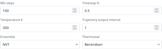
The defaults visible for the phonon-tuned Nequix model are shown below. The model choice and asset state are documented in Choose a Calculator.
Set the trajectory length and sampling interval
Enter the number of propagated steps in MD steps and the integration increment in Timestep fs. The simulated duration is
The defaults, 100 steps and 0.5 fs, produce only 50 fs. That is a stability probe, not equilibrium sampling. The public setup normalizes the number of steps to an integer between 1 and 10,000. A longer scientific trajectory therefore requires repeated, independently documented calls, but the current public operation has no restart state and reinitializes velocities on every call. Separate calls are not a continuous trajectory.
Set Trajectory output interval to the number of MD steps between stored frames. An interval of 10 stores steps 10, 20, and so forth. There is no step-zero frame. The scalar MD trace includes the final step even when the final step is not divisible by the interval, whereas the trajectory does not. For a trajectory that must contain the final structure, choose an interval that divides MD steps.
For systems containing unconstrained hydrogen we recommend starting at 0.5 fs. Reduce the timestep for very stiff bonds, high temperatures, noisy forces, or visible total-energy drift. A larger timestep is justified only by an explicit convergence comparison, preferably an NVE drift test from the same initialized state.
Set temperature and random seed
Temperature K is used every time the command starts, including NVE. Tako discards any incoming velocities, draws mass-weighted Gaussian components from Seed, removes the center-of-mass velocity, and rescales the remaining kinetic energy to the requested temperature using components. The seed therefore changes the initial microscopic state even for deterministic dynamics.
Set Seed explicitly and record it. The same seed reproduces the two deterministic random-number streams used for initialization and, when selected, stochastic thermostat steps. Reproducibility also requires the same structure ordering, masses, constraints, calculator checkpoint, settings, and runtime version.
Choose an effective fixed-cell mode
Set Ensemble to NVE for velocity Verlet without temperature or cell coupling. Set Thermostat and Barostat to None as well so the visible record agrees with the effective algorithm. The temperature field still initializes the velocities; it is not a target maintained during the run.
For fixed-cell NVT, set Ensemble to NVT, choose one thermostat, and leave Barostat at None. The available thermostat choices are Berendsen, Bussi, Langevin, Nose-Hoover, and Andersen. Their control parameters are:
| Thermostat | Operative controls | Interface interpretation |
|---|---|---|
| Berendsen | Temperature K, Taut fs | Deterministic weak coupling; useful for controlled equilibration, not correct canonical fluctuations. |
| Bussi | Temperature K, Taut fs, Seed | Global stochastic velocity rescaling; suitable for canonical sampling after equilibration. |
| Langevin | Temperature K, Friction 1/fs, Seed, Fix COM | Stochastic friction and noise; stronger friction erases dynamical correlations more quickly. |
| Nose-Hoover | Temperature K, Taut fs, T chain, T loop | Deterministic chain thermostat; Fix COM is not applied during its propagation. |
| Andersen | Temperature K, Andersen probability, Seed, Fix COM | Randomizes individual Cartesian velocity components with the per-step probability; it does not collide whole atoms as one event. |
Choosing a non-None barostat while Ensemble is NVT does not move the cell. The runtime ignores that barostat, although the input builder can still request stress. Keep Barostat at None so the settings record is unambiguous and the calculator is not asked for an unused property.
Choose an effective periodic NPT mode
Set Ensemble to NPT only for a fully periodic structure. The following combinations are the supported, unambiguous routes:
| Intended cell dynamics | Thermostat | Barostat | Effective runtime |
|---|---|---|---|
| Berendsen weak coupling | Berendsen | Berendsen | Berendsen temperature scaling and isotropic Berendsen cell scaling |
| Isotropic MTK | Nose-Hoover | MTK isotropic | Nose–Hoover-chain particle and barostat dynamics; cell shape retained |
| Full-cell MTK | Nose-Hoover | MTK full | Coupled particle thermostat and full cell momentum |
| Axis-masked MTK | Nose-Hoover | MTK masked | MTK evolution of the enabled lattice-vector length directions |
The MTK modes use their own Nose–Hoover chains regardless of another thermostat label. Use Nose-Hoover in the dialog so the returned requested settings communicate what the runtime actually does. MTK masked uses MTK x, MTK y, and MTK z from Advanced MD; at least one axis must be enabled. The mask controls lattice-vector length directions in the initial normalized cell basis. It is not a six-component strain mask and does not independently select cell angles.
Avoid the following apparently valid selections:
| Visible selection | Actual behavior |
|---|---|
| NPT + None thermostat + any barostat | Fixed-cell velocity Verlet; the barostat is bypassed. |
| NPT + Nose-Hoover + None barostat | Isotropic MTK NPT; “None” does not prevent cell dynamics. |
| NPT + Bussi, Langevin, or Andersen + None barostat | Berendsen NPT; the requested thermostat is replaced. |
| NPT + Berendsen + an MTK barostat | Berendsen NPT; the MTK selection is overridden. |
The result currently records the normalized selections, not the effective integrator. Select only one of the unambiguous rows above and record it in the calculation notes.
Set pressure and coupling constants
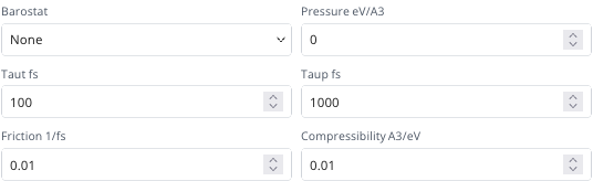
Pressure eV/A3 is the external target pressure. The unit is electronvolts per cubic ångström; . Ambient pressure is approximately zero at the scale shown by the default input. Check sign conventions by a small, known cell perturbation before trusting a new calculator’s NPT behavior.
Compressibility A3/eV controls the response of Berendsen pressure coupling. Taup fs is the pressure-coupling timescale; the default 1000 fs is ten times the default Taut fs of 100 fs. Aggressive pressure coupling can collapse or oscillate a cell even when fixed-cell dynamics is stable. Begin with a short NVT run, verify the stress, then introduce slow cell coupling.
Taut fs controls Berendsen, Bussi, and the characteristic Nose–Hoover thermostat mass. Friction 1/fs is used only by Langevin dynamics. Values displayed for other modes remain inert; the interface does not hide them when a different mode is selected.
Use Advanced MD
Expand Advanced MD only after selecting the effective algorithm.
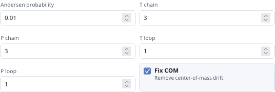
Andersen probability is a per-Cartesian-component, per-step redraw probability. T chain and T loop control the Nose–Hoover particle thermostat chain and its substeps. P chain and P loop apply to MTK pressure chains. The chain and loop counts are normalized to integers from 1 through 32.
Fix COM requests removal of center-of-mass drift during Berendsen, Bussi, Langevin, and Andersen propagation. Initial center-of-mass motion is always removed, even when the box is cleared. The option is not consulted during Nose–Hoover-chain or MTK propagation, so the checkbox does not constrain COM motion in those modes.

The three MTK axis options apply only to MTK masked. They do not affect Berendsen, isotropic MTK, or full MTK.
Start and monitor the calculation
Choose Start after checking that the visible combination appears in one of the unambiguous tables above. The Console reports the requested step count, timestep, temperature, ensemble, thermostat, and barostat. These log labels are requested settings, not an independently resolved effective-integrator report.
During a successful run, Tako streams stored trajectory frames. The viewer can play those frames and plot their potential-energy values. Smooth playback does not confirm numerical stability: watch for sudden geometry changes, rapid cell deformation, a monotonic total-energy drift in NVE, persistent temperature displacement, and discontinuities introduced by the output interval.
Open the outputs
The calculation folder contains the following MD-specific artifacts when their source data is available:
| Artifact | Content and boundary |
|---|---|
result.json | Complete public result object: final scalar values, stored frames, full scalar trace, requested settings, final atoms, and a simple XYZ serialization. |
md.traj | Stored trajectory frames at the selected output interval; no step-zero frame and possibly no final frame. |
md_trace.json | Scalar entry for every stored interval and always the final step; energies and temperature are present. Its current cell matrices are internal Bohr values, unlike frame cells in ångström. |
energy_trace.json | Potential energy derived from stored frames, not from every entry in md_trace.json; it can omit the final step. |
The result does not expose velocities, momenta, pressure, volume, density, stress, enthalpy, conserved extended-system energy, thermostat work, barostat work, autocorrelation analysis, or restart state. Do not infer those quantities from an animation. The generic frame object also contains optimization-shaped fmax and maxstep fields set to zero; they are compatibility fields, not MD observables.
Validate before interpreting
A completed run records that execution finished, not that the result is valid. Timestep and drift checks, equilibration criteria, autocorrelation and effective sample size, and per-ensemble diagnostics are covered in Molecular Dynamics: Statistics and Validation; start with its acceptance checklist before reporting any number from this run.
Diagnose failures
| Observation | Likely cause | Interface response |
|---|---|---|
| Energy or temperature diverges within a few steps | overlap, poor optimization, timestep too large, or noisy forces | Stop; optimize, reduce Timestep fs, and test NVE. |
| NVE total energy drifts monotonically | timestep/model numerical error or constraint work | Halve Timestep fs and compare the drift slope. |
| Temperature is displaced immediately for a constrained system | initializer used rather than constrained degrees of freedom | Treat the first segment as initialization; verify with a short run and reconsider constraints. |
| NPT reports fixed cell | Thermostat is None, causing velocity-Verlet routing | Select an unambiguous NPT row. |
| NPT cell moves although Barostat says None | Nose-Hoover routes to isotropic MTK | Select and record MTK isotropic explicitly. |
| MTK fails before propagation | constraints, missing cell/stress, or all masked axes disabled | Remove incompatible constraints, verify periodic cell/stress, and enable an axis. |
| Cell collapses or oscillates | stress sign/model failure or aggressive pressure coupling | Return to NVT; validate stress; increase Taup fs and reduce timestep. |
| Final trace step has no trajectory frame | output interval does not divide step count | Choose a divisor of MD steps when the final frame is required. |
| Repeating the call does not continue the trajectory | public restart state is absent and velocities are regenerated | Treat every call as a new trajectory; do not concatenate as continuous dynamics. |
Record the starting structure and atom order, calculator identifier and checkpoint, all visible MD and advanced values, seed, constraints, periodicity, total duration, frame interval, runtime version, and every convergence comparison. The deeper interpretation and reporting checklist are in Molecular Dynamics.